Baseline Model

Establish a reproducible TF‑IDF + Logistic Regression benchmark for Twitter‑airline sentiment.

Text column → clean_text
Target label → airline_sentiment (negative, neutral, positive)
Train / validation / test = 70 / 15 / 15 (stratified)
Persist artefacts to models/

Notebook Outline

Load Processed Data & Train-Test Split
Majority-class reference
TF-IDF + Logistic Regression pipeline
Validation performance
5-fold stratified CV on all data
Persisted Artifacts
Key Takeaway

Code

# Imports
from __future__ import annotations

import json
from pathlib import Path
import matplotlib.pyplot as plt

import joblib
import pandas as pd
from sklearn.model_selection import (
    train_test_split,
    cross_val_score,
    StratifiedKFold,
)
from sklearn.pipeline import Pipeline
from sklearn.feature_extraction.text import TfidfVectorizer
from sklearn.linear_model import LogisticRegression
from sklearn.metrics import (
    classification_report,
    ConfusionMatrixDisplay,
    accuracy_score,
    f1_score
)

# Detect project root (folder that contains "data/")
ROOT_DIR = Path.cwd().parent  

# Define core directories
DATA_DIR      = ROOT_DIR / "data"
PROC_DATA_DIR = DATA_DIR / "processed"
MODELS_DIR    = ROOT_DIR / "models"
REPORT_DIR    = ROOT_DIR / "reports" / "figs_04"

MODELS_DIR.mkdir(exist_ok=True)
REPORT_DIR.mkdir(parents=True, exist_ok=True)

# Locate tweets.parquet (processed > raw fallback)
PARQUET_PATH = (
    PROC_DATA_DIR / "tweets.parquet"
    if (PROC_DATA_DIR / "tweets.parquet").exists()
    else DATA_DIR / "tweets.parquet"
)
assert PARQUET_PATH.exists(), f"Missing parquet at {PARQUET_PATH}"

print(f"Project root  : {ROOT_DIR}")
print(f"Parquet source : {PARQUET_PATH.relative_to(ROOT_DIR)}")

Project root  : C:\Projects\twitter-airline-analysis
Parquet source : data\processed\tweets.parquet

1. Load Processed Data & Train-Test Split

We keep raw string labels (airline_sentiment); scikit-learn encodes them internally.

Code

df = pd.read_parquet(PARQUET_PATH)

# Assert expected columns are present
required_cols = {"clean_text", "airline_sentiment"}
missing = required_cols - set(df.columns)
assert not missing, f"Missing columns: {missing}"

# Sanity: no nulls in features / target
assert df.clean_text.isna().sum() == 0
assert df.airline_sentiment.isna().sum() == 0

# Train / valid / test = 70 / 15 / 15
X_train, X_temp, y_train, y_temp = train_test_split(
    df.clean_text,
    df.airline_sentiment,
    test_size=0.30,
    stratify=df.airline_sentiment,
    random_state=42,
)
X_valid, X_test, y_valid, y_test = train_test_split(
    X_temp,
    y_temp,
    test_size=0.50,
    stratify=y_temp,
    random_state=42,
)

print(
    f"Splits → train:{len(X_train)}  valid:{len(X_valid)}  test:{len(X_test)}"
)

Splits → train:10248  valid:2196  test:2196

2. Majority‑class reference

Majority‑class accuracy: 0.627
(Always predicting negative is correct 62.7 % of the time.)

Code

majority_acc = y_train.value_counts(normalize=True).max()
print(f"Majority‑class accuracy: {majority_acc:.3f}")

Majority‑class accuracy: 0.627

3. TF‑IDF + Logistic Regression pipeline

Bi‑gram coverage, minimal regularisation tuning, and class_weight='balanced' to counter the 63 % negative skew.

Code

pipe_lr = Pipeline(
    [
        (
            "tfidf",
            TfidfVectorizer(
                ngram_range=(1, 2),
                min_df=2,
                max_features=50_000,
            ),
        ),
        (
            "clf",
            LogisticRegression(
                max_iter=2_000,
                n_jobs=-1,
                class_weight="balanced",
            ),
        ),
    ]
)

pipe_lr.fit(X_train, y_train)

Pipeline(steps=[('tfidf',
                 TfidfVectorizer(max_features=50000, min_df=2,
                                 ngram_range=(1, 2))),
                ('clf',
                 LogisticRegression(class_weight='balanced', max_iter=2000,
                                    n_jobs=-1))])

In a Jupyter environment, please rerun this cell to show the HTML representation or trust the notebook.
On GitHub, the HTML representation is unable to render, please try loading this page with nbviewer.org.

4. Validation performance

Metric	Score
Accuracy	0.788
Macro F1	0.741
Weighted F1	0.792

The model is strongest on the negative class (precision ≈ 0.89) and weakest on neutral—an expected pattern given the class imbalance.

Code

print(
    classification_report(
        y_valid,
        pipe_lr.predict(X_valid),
        digits=3,
        target_names=["neg", "neu", "pos"],
    )
)

              precision    recall  f1-score   support

         neg      0.888     0.836     0.862      1376
         neu      0.590     0.703     0.642       465
         pos      0.728     0.710     0.719       355

    accuracy                          0.788      2196
   macro avg      0.736     0.750     0.741      2196
weighted avg      0.799     0.788     0.792      2196

5. 5‑fold stratified CV on all data

Cross-Validated Macro F1: 0.749 ± 0.007

The low standard deviation indicates the baseline is stable across folds.

Code

cv = StratifiedKFold(n_splits=5, shuffle=True, random_state=42)

cv_scores = cross_val_score(
    pipe_lr,
    df.clean_text,
    df.airline_sentiment,
    cv=cv,
    scoring="f1_macro",
    n_jobs=-1,
)

print(f"CV F1_macro = {cv_scores.mean():.3f} ± {cv_scores.std():.3f}")

CV F1_macro = 0.749 ± 0.007

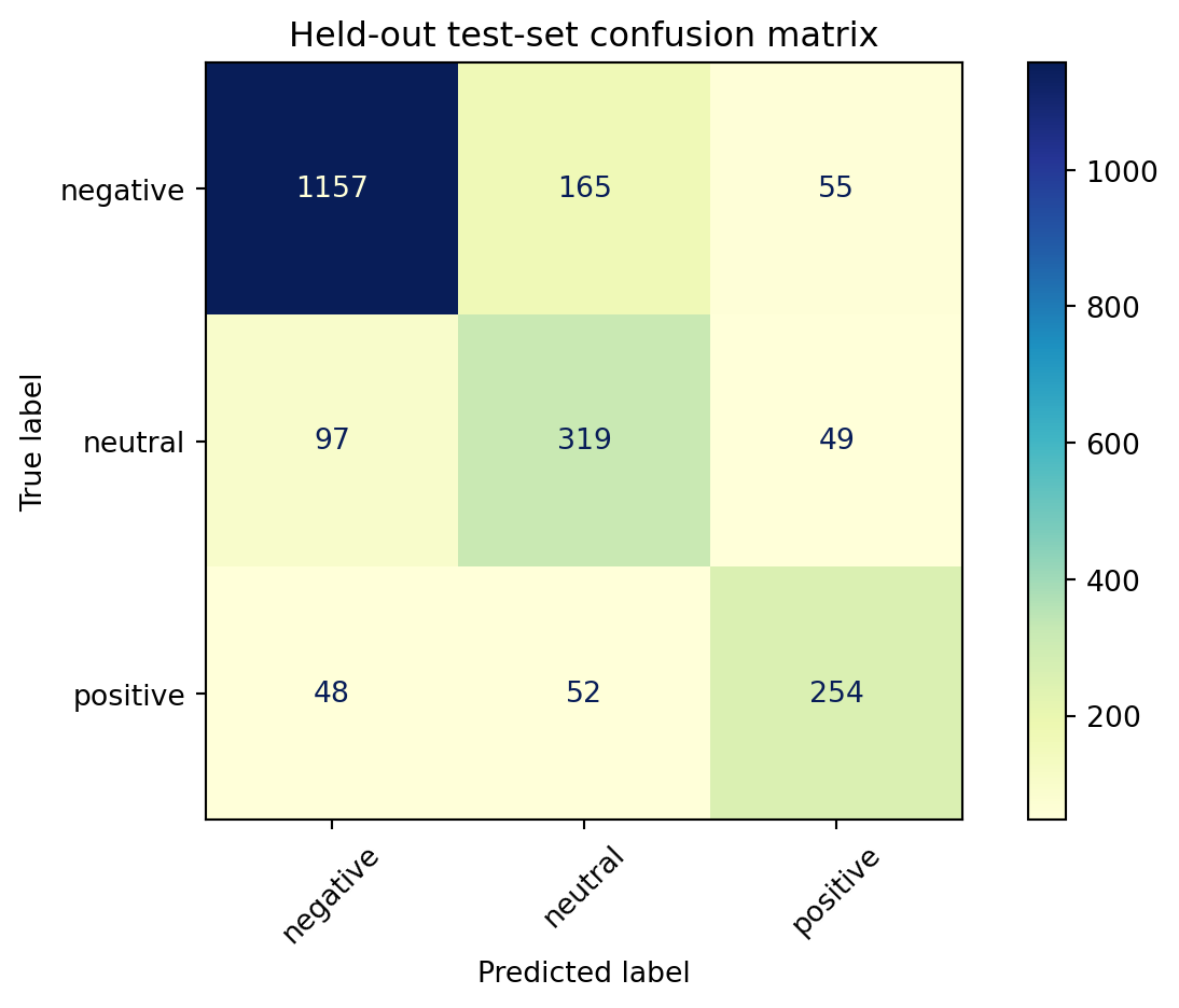
Held-Out Test Set Confusion Matrix

The confusion matrix visually confirms the model’s strengths and areas for improvement:

Negative Class: Excellent recall and precision.
Neutral Class: Frequent confusion with both negative and positive classes indicates difficulty capturing neutrality.

(Matrix figure saved as reports/figs_04/conf_matrix.png.)

Code

# Held‑out predictions  
y_pred = pipe_lr.predict(X_test)   # X_test comes from the earlier split cell

report_dict = classification_report(
    y_test, y_pred,
    target_names=["negative", "neutral", "positive"],
    output_dict=True,
    zero_division=0       
)

# tidy DataFrame, keep only precision/recall/f1
metrics_df = (
    pd.DataFrame(report_dict)
      .T                                   # classes as rows
      .loc[["negative", "neutral", "positive", "weighted avg"],  # row order
           ["precision", "recall", "f1-score"]]
      .rename(index={"weighted avg": "weighted"})                # shorter name
      .round(3)
)

display(metrics_df)

overall = pd.Series({
    "accuracy":      accuracy_score(y_test, y_pred),
    "weighted‑F1":   f1_score(y_test, y_pred, average="weighted")
}).round(3)

print("\nOverall:", overall.to_dict())

disp = ConfusionMatrixDisplay.from_predictions(
    y_test, y_pred,
    labels=["negative", "neutral", "positive"],
    cmap="YlGnBu", xticks_rotation=45, colorbar=True
)

plt.title("Held‑out test‑set confusion matrix")
plt.tight_layout()
plt.savefig(REPORT_DIR / "conf_matrix.png", dpi=150)
plt.show()

	precision	recall	f1-score
negative	0.889	0.840	0.864
neutral	0.595	0.686	0.637
positive	0.709	0.718	0.713
weighted	0.798	0.788	0.792


Overall: {'accuracy': 0.788, 'weighted‑F1': 0.792}

6. Persisted Artifacts

Model: models/logreg_tfidf.joblib
Cross-Validation Scores: models/cv_logreg.json

Code

MODEL_PATH = MODELS_DIR / "logreg_tfidf.joblib"
CV_PATH    = MODELS_DIR / "cv_logreg.json"

joblib.dump(pipe_lr, MODEL_PATH)
print(f"Saved model → {MODEL_PATH.relative_to(ROOT_DIR)}")

with CV_PATH.open("w") as fp:
    json.dump({"f1_macro": cv_scores.tolist()}, fp, indent=2)
print(f"Saved CV scores → {CV_PATH.relative_to(ROOT_DIR)}")

Saved model → models\logreg_tfidf.joblib
Saved CV scores → models\cv_logreg.json

7. Key Takeaway

Baseline (majority class) caps out at 62.7 % accuracy.
TF‑IDF + Logistic Regression lifts validation accuracy to 78.8 % and macro F1 to 0.74.
5‑fold CV confirms robustness (0.749 ± 0.007 macro F1).
Confusion matrix shows excellent precision for the negative class but persistent confusion between neutral and both extremes.
With class‑weight balancing and bigram coverage, a classical model already delivers a +16 pp accuracy gain over the baseline—good enough for a production fallback while we prototype transformer models in Milestone 5.

	steps	[('tfidf', ...), ('clf', ...)]
	transform_input	None
	memory	None
	verbose	False

	input	'content'
	encoding	'utf-8'
	decode_error	'strict'
	strip_accents	None
	lowercase	True
	preprocessor	None
	tokenizer	None
	analyzer	'word'
	stop_words	None
	token_pattern	'(?u)\\b\\w\\w+\\b'
	ngram_range	(1, ...)
	max_df	1.0
	min_df	2
	max_features	50000
	vocabulary	None
	binary	False
	dtype	<class 'numpy.float64'>
	norm	'l2'
	use_idf	True
	smooth_idf	True
	sublinear_tf	False

	penalty	'l2'
	dual	False
	tol	0.0001
	C	1.0
	fit_intercept	True
	intercept_scaling	1
	class_weight	'balanced'
	random_state	None
	solver	'lbfgs'
	max_iter	2000
	multi_class	'deprecated'
	verbose	0
	warm_start	False
	n_jobs	-1
	l1_ratio	None

Notebook Outline

1. Load Processed Data & Train-Test Split

2. Majority‑class reference

3. TF‑IDF + Logistic Regression pipeline

4. Validation performance

5. 5‑fold stratified CV on all data

Held-Out Test Set Confusion Matrix

6. Persisted Artifacts

7. Key Takeaway

3. TF‑IDF + Logistic Regression pipeline