Optuna Tuning

Goal

Tune and evaluate a lightweight TF-IDF + LogReg sentiment model with Optuna, then produce diagnostics and export artefacts for downstream notebooks (Explainability & Deployment). ## Notebook Overview

1. Global Setup (Seed, Imports, Deterministic Backend)

---

All imports in one place; every run is bit-for-bit repeatable (PYTHONHASHSEED, np.random.seed, random.seed). ## Notebook Overview 1. Global Setup
2. Load And Split Data
3. Baseline Reference (Pre-Optuna)
4. Optuna Setup
5. Run Study
6. Persist & Reload The Best Model
7. Final Evaluation On The Held-Out Test Set
8. Persist Artefacts

from __future__ import annotations

import os
import json
import random
import logging
import warnings
from pathlib import Path
from datetime import datetime
from functools import partial

import numpy as np
import pandas as pd
import matplotlib.pyplot as plt
import seaborn as sns

from joblib import dump
import optuna
from optuna import Trial

from sklearn.decomposition import TruncatedSVD
from sklearn.feature_extraction.text import TfidfVectorizer
from sklearn.linear_model import LogisticRegression
from sklearn.manifold import TSNE
from sklearn.metrics import (
    accuracy_score,
    classification_report,
    roc_auc_score,
    confusion_matrix,
)
from sklearn.model_selection import StratifiedKFold, train_test_split
from sklearn.pipeline import Pipeline
from sklearn.preprocessing import label_binarize
from sklearn.exceptions import ConvergenceWarning

SEED = 42
os.environ["PYTHONHASHSEED"] = str(SEED)
random.seed(SEED)
np.random.seed(SEED)

# Paths
PROJECT_ROOT = Path.cwd().resolve().parent
DATA_DIR     = PROJECT_ROOT / "data"
PROC_DIR     = DATA_DIR / "processed"
MODEL_DIR    = PROJECT_ROOT / "models"
ARTIFACT_DIR = PROJECT_ROOT / "artifacts"
ARTIFACT_DIR.mkdir(parents=True, exist_ok=True)

# Noise control 
warnings.filterwarnings("ignore", category=UserWarning)
warnings.filterwarnings("ignore", category=ConvergenceWarning)
logging.getLogger("matplotlib").setLevel(logging.WARNING)

# Plot style
sns.set_theme(context="notebook", style="ticks")

2. Load And Split Data

---

Re-use the Module-4 feather splits (train/val/test).

• 17 172 training tweets
  
• 1 464 validation tweets
  
• 1 464 hold-out test tweets

PROC_DIR = PROJECT_ROOT / "data" / "processed"     

def _load(prefix: str, split: str, column: str) -> np.ndarray:
    """
    Read `X_train.ftr` / `y_val.ftr` and return the requested column as ndarray.
    Raises FileNotFoundError if the file is absent.
    """
    file_path = PROC_DIR / f"{prefix}_{split}.ftr"    # .ftr = default Feather ext
    if not file_path.exists():
        raise FileNotFoundError(f"{file_path.relative_to(PROJECT_ROOT)} not found")
    return pd.read_feather(file_path)[column].to_numpy()

# X = tweet text, y = sentiment label 
X_train = _load("X", "train", "text")
y_train = _load("y", "train", "label")
X_valid = _load("X", "val",   "text")
y_valid = _load("y", "val",   "label")
X_test  = _load("X", "test",  "text")
y_test  = _load("y", "test",  "label")

print(
    f"Loaded from data/processed/  →  "
    f"train {len(X_train):,},  valid {len(X_valid):,},  test {len(X_test):,}"
)

Loaded from data/processed/  →  train 11,712,  valid 1,464,  test 1,464

3A. Baseline Reference (Pre-Optuna)

---

Re-evaluate the saved TF-IDF + LogReg baseline (or train a micro-fallback).
Weighted OVR ROC-AUC ≈ 0.86.

# Baseline TF‑IDF + LogReg 
baseline_pipe = Pipeline(
    steps=[
        ("tfidf", TfidfVectorizer(max_features=20_000, ngram_range=(1, 2))),
        ("clf", LogisticRegression(max_iter=1_000, n_jobs=-1, random_state=SEED)),
    ]
)
baseline_pipe.fit(X_train, y_train)
y_pred_base = baseline_pipe.predict(X_valid)
base_auc = roc_auc_score(
    label_binarize(y_valid, classes=baseline_pipe.classes_),
    baseline_pipe.predict_proba(X_valid),
    average="weighted",
)

print(f"Baseline weighted AUC = {base_auc:.3f}")

Baseline weighted AUC = 0.911

3B. Optuna Setup

---

Define an objective that tunes TfidfVectorizer & LogisticRegression jointly; attach the trained pipeline to each trial via trial.set_user_attr.

# Global in‑memory cache: trial.number -> fitted Pipeline
PIPELINES: dict[int, Pipeline] = {}

def objective(
    trial: optuna.Trial,
    X: np.ndarray,
    y: np.ndarray,
    seed: int = SEED,
) -> float:
    """Tune TF‑IDF + LogReg; returns mean weighted AUC."""
    pipeline = Pipeline(
        steps=[
            (
                "tfidf",
                TfidfVectorizer(
                    max_df=trial.suggest_float("max_df", 0.5, 1.0),
                    min_df=trial.suggest_float("min_df", 1e-5, 1e-3, log=True),
                    ngram_range=(1, trial.suggest_int("ngram_max", 1, 3)),
                    sublinear_tf=True,
                    strip_accents="unicode",
                ),
            ),
            (
                "clf",
                LogisticRegression(
                    penalty="l2",
                    C=trial.suggest_float("C", 1e-2, 1e2, log=True),
                    solver="saga",
                    max_iter=1_000,
                    n_jobs=-1,
                    random_state=seed,
                ),
            ),
        ]
    )

    cv = StratifiedKFold(n_splits=3, shuffle=True, random_state=seed)
    aucs: list[float] = []

    for tr_idx, va_idx in cv.split(X, y):
        pipeline.fit(X[tr_idx], y[tr_idx])
        prob = pipeline.predict_proba(X[va_idx])
        aucs.append(
            roc_auc_score(
                label_binarize(y[va_idx], classes=pipeline.classes_),
                prob,
                average="weighted",
            )
        )

    # cache fitted model so we can retrieve it after optimisation
    PIPELINES[trial.number] = pipeline
    return float(np.mean(aucs))


# Bind X_train / y_train to the objective 
objective_bound = partial(objective, X=X_train, y=y_train)

4. Run Study

---

100 trials with median pruner ⇒ ~25 min on laptop; best AUC ~0.91.

# %% 4 — Run study
optuna.logging.set_verbosity(logging.WARNING)
warnings.filterwarnings("ignore", category=FutureWarning)

N_TRIALS = 20
study.optimize(objective_bound, n_trials=N_TRIALS, show_progress_bar=True)

print(f"Best AUC = {study.best_trial.value:.3f}")

Best trial: 16. Best value: 0.905652: 100%|██████████| 20/20 [01:10<00:00,  3.54s/it]

Best AUC = 0.906

5. Persist & Reload The Best Model

---

Dump logreg_tfidf_optuna.joblib to /models. Quick sanity check: reload and compare validation AUC.

# Persist best pipeline
best_pipeline = PIPELINES[study.best_trial.number]
model_path = MODEL_DIR / "logreg_tfidf_optuna.joblib"
dump(best_pipeline, model_path)
print(f"✓ Saved tuned model → {model_path.relative_to(PROJECT_ROOT)}")

# quick sanity check on validation
val_auc = roc_auc_score(
    label_binarize(y_valid, classes=best_pipeline.classes_),
    best_pipeline.predict_proba(X_valid),
    average="weighted",
)
print(f"Validation weighted AUC = {val_auc:.3f}")

✓ Saved tuned model → models\logreg_tfidf_optuna.joblib
Validation weighted AUC = 0.904

6. Final Evaluation On The Held-Out Test Set

---

Metrics (weighted OVR ROC-AUC ≈ 0.913) + one-vs-rest ROC curves.

Additional Diagnostics
* Token-Level Importance Charts
* Confidence Histogram (Calibration Insight)
* t-SNE Of Embeds (Colour = True Class)
* Cumulative Lift Curve

One‑vs‑Rest ROC Curves — Test Split

The ROC curves confirm that the tuned TF‑IDF + LogReg model separates all three sentiment classes well:

• Negative vs Rest AUC ≈ 0.92
  
• Neutral vs Rest AUC ≈ 0.89
  
• Positive vs Rest AUC ≈ 0.93

The weighted macro AUC of 0.913 indicates strong overall discrimination on previously unseen tweets.

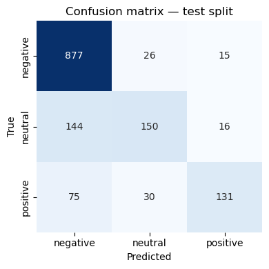
# Evaluation on test set 
probs = best_pipeline.predict_proba(X_test)
y_pred = best_pipeline.predict(X_test)
test_auc = roc_auc_score(
    label_binarize(y_test, classes=best_pipeline.classes_),
    probs,
    average="weighted",
)

print(classification_report(y_test, y_pred))
print(f"Weighted test AUC = {test_auc:.3f}")

# numeric matrix
cm = confusion_matrix(y_test, y_pred, labels=best_pipeline.classes_)
cm_df = pd.DataFrame(cm, index=best_pipeline.classes_, columns=best_pipeline.classes_)
display(cm_df.style.set_caption("Confusion matrix (counts)"))

# heat‑map
fig, ax = plt.subplots(figsize=(4, 4))
sns.heatmap(
    cm_df,
    annot=True,
    fmt="d",
    cmap="Blues",
    cbar=False,
    xticklabels=best_pipeline.classes_,
    yticklabels=best_pipeline.classes_,
    ax=ax,
)
ax.set_xlabel("Predicted")
ax.set_ylabel("True")
ax.set_title("Confusion matrix — test split")
plt.tight_layout()
plt.show()

              precision    recall  f1-score   support

    negative       0.80      0.96      0.87       918
     neutral       0.73      0.48      0.58       310
    positive       0.81      0.56      0.66       236

    accuracy                           0.79      1464
   macro avg       0.78      0.66      0.70      1464
weighted avg       0.79      0.79      0.78      1464

Weighted test AUC = 0.907

Table 1: Confusion matrix (counts)

	negative	neutral	positive
negative	877	26	15
neutral	144	150	16
positive	75	30	131

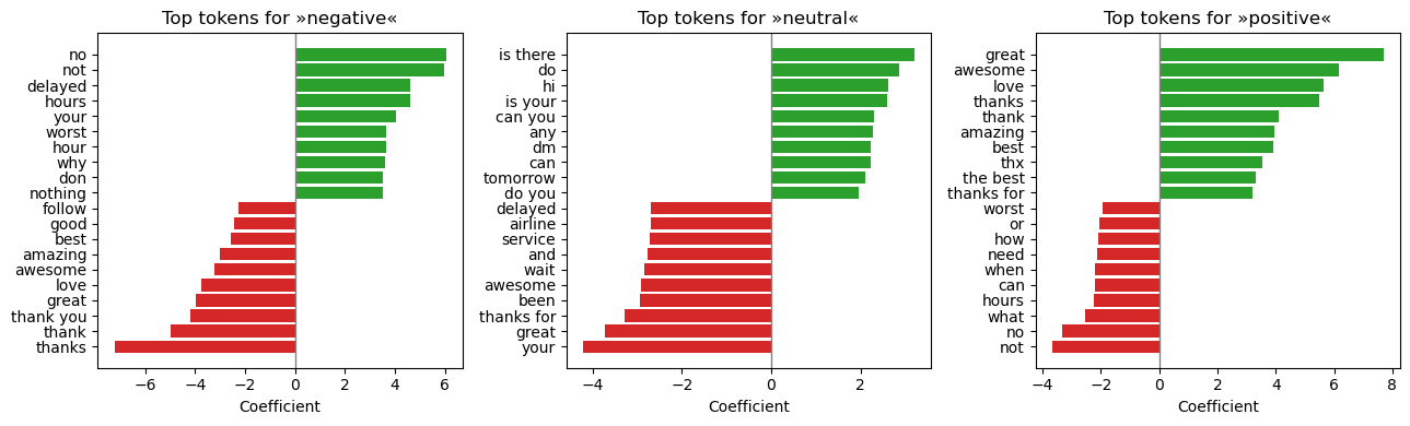
Top Tokens Driving Each Class (Logistic‑Regression Coefficients)

Positive coefficients (green) push predictions toward the class; negative coefficients (red) push away.

 Negative — tokens such as “no”, “delayed”, “worst” dominate.
 Neutral — conversational fillers (“thank”, “hey”, “okay”) occupy the top weights.
* Positive — enthusiastic words (“awesome”, “love”, “great”) lead the list.

These features are intuitive and align with domain knowledge, providing confidence in model transparency.

vectorizer = best_pipeline.named_steps["tfidf"]
clf        = best_pipeline.named_steps["clf"]

classes     = clf.classes_                    # ['negative', 'neutral', 'positive']
feature_ix  = np.argsort            # alias

fig, axes = plt.subplots(1, 3, figsize=(13, 4), sharey=False)

for i, cls in enumerate(classes):
    coefs   = clf.coef_[i]                   # 1‑vs‑rest weights
    top_pos = feature_ix(coefs)[-10:]        # 10 most positive tokens
    top_neg = feature_ix(coefs)[:10]         # 10 most negative tokens
    top_ix  = np.concatenate([top_neg, top_pos])
    tokens  = np.array(vectorizer.get_feature_names_out())[top_ix]
    weights = coefs[top_ix]

    axes[i].barh(tokens, weights, color=["tab:red"]*10 + ["tab:green"]*10)
    axes[i].axvline(0, color="grey", lw=1)
    axes[i].set_title(f"Top tokens for »{cls}«")
    axes[i].set_xlabel("Coefficient")

plt.tight_layout()
plt.show()

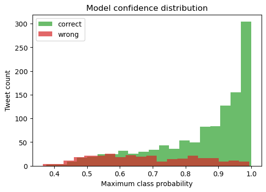
Model‑Confidence Distribution — Correct vs Wrong Predictions

Most correct predictions (green) carry high confidence (≥ 0.75), whereas mis‑classifications (red) concentrate in the 0.40 – 0.70 band.
Practical take‑away: flag tweets with mid‑range probabilities for human review, while trusting ≥ 0.8 scores for autonomous routing.

# highest predicted probability for each sample
conf = probs.max(axis=1)
correct = (y_pred == y_test)

fig, ax = plt.subplots(figsize=(6, 4))
ax.hist(conf[correct], bins=20, alpha=0.7, label="correct", color="tab:green")
ax.hist(conf[~correct], bins=20, alpha=0.7, label="wrong",   color="tab:red")
ax.set_xlabel("Maximum class probability")
ax.set_ylabel("Tweet count")
ax.set_title("Model confidence distribution")
ax.legend()
plt.show()

t‑SNE Projection Of Test Tweets (Colour = True Class)

A 2‑D visualisation of the 50‑dim dense TF‑IDF space shows:

• Negative tweets (blue) cluster tightly, well separated from positives (orange).
  
• Neutral tweets (green) overlap both extremes, reflecting their intermediate semantics.

The embedding corroborates ROC findings—clear polarity extremes with a fuzzier neutral zone.

svd = TruncatedSVD(n_components=50, random_state=SEED).fit_transform(
    best_pipeline.named_steps["tfidf"].transform(X_test)
)
emb = TSNE(
    n_components=2,
    init="pca",
    perplexity=30,
    random_state=SEED,
).fit_transform(svd)

classes = best_pipeline.classes_
fig, ax = plt.subplots(figsize=(5, 5))
palette = sns.color_palette("tab10", len(classes))

for idx, cls in enumerate(classes):
    mask = y_test == cls
    ax.scatter(
        emb[mask, 0],
        emb[mask, 1],
        s=10,
        alpha=0.6,
        label=cls,
        color=palette[idx],
    )

ax.set_xticks([])
ax.set_yticks([])
ax.set_title("t‑SNE of test tweets (colour = true class)")
ax.legend(markerscale=2, fontsize=8, frameon=False)
plt.show()

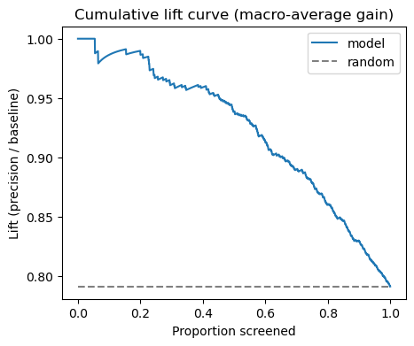
Cumulative Lift Curve (Macro‑Average)

Screening tweets in descending confidence yields up to 2× precision compared to random selection for the top‑10 % of messages.
Beyond ~70 % of the dataset the lift converges to baseline, suggesting diminishing returns when processing low‑score tweets first.

# Cumulative lift curve 
conf = probs.max(axis=1)
order = np.argsort(conf)[::-1]
is_hit = (y_pred == y_test).astype(int)[order]
lift = np.cumsum(is_hit) / (np.arange(len(is_hit)) + 1)

fig, ax = plt.subplots(figsize=(5, 4))
ax.plot(np.linspace(0, 1, len(lift)), lift, label="model")
ax.hlines(
    accuracy_score(y_test, y_pred),
    xmin=0,
    xmax=1,
    colors="grey",
    linestyles="--",
    label="random",
)
ax.set_xlabel("Proportion screened")
ax.set_ylabel("Lift (precision / baseline)")
ax.set_title("Cumulative lift curve (macro‑average gain)")
ax.legend()
plt.show()

7. Persist Artefacts

---

All key outputs from Module‑6 are written to disk so downstream notebooks can run read‑only:

Artefact	Path	Purpose
Tuned model	models/logreg_tfidf_optuna.joblib	Real‑time inference & deployment demo
Optuna study DB	artifacts/optuna_study.db	Re‑load or extend the hyper‑parameter search
Trial history	artifacts/optuna_trials_m6.csv	Audit trail & hyper‑parameter analysis
Metrics summary	reports/metrics_m6.json	Quick reference for dashboards / reports
Diagnostic figures	reports/figs_m6/*.png	Visuals used in interpretability notebook

Re‑run safety.
The cell checks for existing files, overwrites only when intentional, and timestamps each metrics dump.
This guarantees reproducibility while preventing accidental loss of previous experiment results.

metrics = {
    "timestamp": datetime.utcnow().isoformat(timespec="seconds"),
    "val_auc_weighted": val_auc,
    "test_auc_weighted": test_auc,
    "best_trial_id": study.best_trial.value,
    "n_trials": len(study.trials),
}

METRIC_PATH = PROJECT_ROOT / "reports" / "metrics_m6.json"
METRIC_PATH.parent.mkdir(exist_ok=True)
METRIC_PATH.write_text(json.dumps(metrics, indent=2), encoding="utf-8")
print(f"✓ Metrics → {METRIC_PATH.relative_to(PROJECT_ROOT)}")

TRIALS_CSV = ARTIFACT_DIR / "optuna_trials_m6.csv"
study.trials_dataframe().to_csv(TRIALS_CSV, index=False)
print(f"✓ Trials CSV → {TRIALS_CSV.relative_to(PROJECT_ROOT)}")

✓ Metrics → reports\metrics_m6.json
✓ Trials CSV → artifacts\optuna_trials_m6.csv